Week 3 — ARMA Models

Autoregressive Moving Average (ARMA) models are the building blocks of time-series forecasting. This notebook covers AR, MA, and ARMA processes, their properties, and how to identify them from data.

import matplotlib as mpl
import matplotlib.pyplot as plt
import numpy as np

# Edinburgh palette
UOE_RED   = '#7A2318'
UOE_GOLD  = '#B8860B'
UOE_BLUE  = '#2a78d6'
UOE_GREY  = '#52514e'
COLOURS   = [UOE_RED, UOE_BLUE, UOE_GOLD, '#2ca02c', '#9467bd', '#e377c2']

mpl.rcParams.update({
    'figure.figsize': (10, 5),
    'axes.prop_cycle': mpl.cycler(color=COLOURS),
    'axes.spines.top': False, 'axes.spines.right': False,
    'axes.labelsize': 12, 'axes.titlesize': 14,
    'font.size': 11, 'legend.fontsize': 10,
    'lines.linewidth': 2,
})
print("Plotting style set ✓")

Plotting style set ✓

3.1 The AR(1) Process

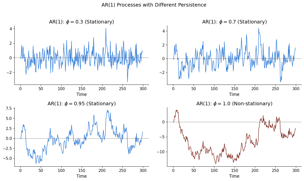
\[y_t = c + \phi y_{t-1} + \varepsilon_t, \quad \varepsilon_t \sim WN(0, \sigma^2)\]

Stationarity requires \(|\phi| < 1\).

np.random.seed(42)
T = 300
eps = np.random.normal(0, 1, T)

phi_values = [0.3, 0.7, 0.95, 1.0]
fig, axes = plt.subplots(2, 2, figsize=(12, 7))

for ax, phi in zip(axes.flat, phi_values):
    y = np.zeros(T)
    for t in range(1, T):
        y[t] = phi * y[t-1] + eps[t]
    ax.plot(y, color=UOE_RED if phi >= 1 else UOE_BLUE, lw=1.2)
    ax.axhline(0, ls='--', color=UOE_GREY, lw=0.8)
    status = 'Non-stationary' if phi >= 1 else 'Stationary'
    ax.set_title(f'AR(1): $\\phi = {phi}$ ({status})')
    ax.set_xlabel('Time')

plt.suptitle('AR(1) Processes with Different Persistence', fontsize=14, y=1.02)
plt.tight_layout()
plt.show()

3.2 The MA(1) Process

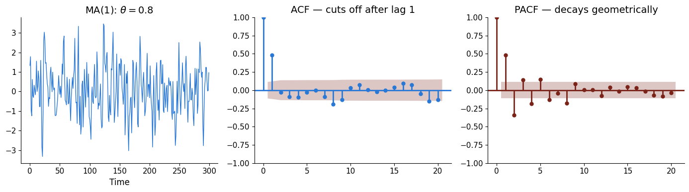
\[y_t = \mu + \varepsilon_t + \theta \varepsilon_{t-1}\]

MA processes are always stationary. The ACF cuts off after lag \(q\).

from statsmodels.graphics.tsaplots import plot_acf, plot_pacf
from statsmodels.tsa.arima_process import ArmaProcess

# MA(1) with theta = 0.8
ma1 = ArmaProcess(ar=[1], ma=[1, 0.8])
np.random.seed(10)
y_ma = ma1.generate_sample(nsample=300)

fig, (ax1, ax2, ax3) = plt.subplots(1, 3, figsize=(14, 4))
ax1.plot(y_ma, color=UOE_BLUE, lw=1)
ax1.set_title('MA(1): $\\theta = 0.8$')
ax1.set_xlabel('Time')

plot_acf(y_ma, lags=20, ax=ax2, color=UOE_BLUE, vlines_kwargs={'color': UOE_BLUE})
ax2.set_title('ACF — cuts off after lag 1')

plot_pacf(y_ma, lags=20, ax=ax3, color=UOE_RED, vlines_kwargs={'color': UOE_RED})
ax3.set_title('PACF — decays geometrically')

plt.tight_layout()
plt.show()

3.3 ARMA(p, q) — Combining AR and MA

\[y_t = c + \sum_{i=1}^{p} \phi_i y_{t-i} + \varepsilon_t + \sum_{j=1}^{q} \theta_j \varepsilon_{t-j}\]

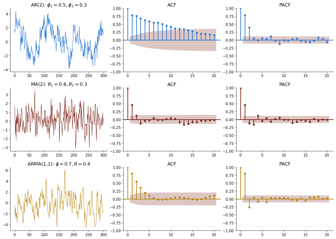
Identification rules:

Model	ACF	PACF
AR(p)	Decays	Cuts off after lag \(p\)
MA(q)	Cuts off after lag \(q\)	Decays
ARMA(p,q)	Decays	Decays

from statsmodels.graphics.tsaplots import plot_acf, plot_pacf
# Theoretical ACF/PACF for different ARMA models
from statsmodels.tsa.arima_process import ArmaProcess

models = {
    'AR(2): $\\phi_1=0.5, \\phi_2=0.3$': ArmaProcess(ar=[1, -0.5, -0.3], ma=[1]),
    'MA(2): $\\theta_1=0.6, \\theta_2=0.3$': ArmaProcess(ar=[1], ma=[1, 0.6, 0.3]),
    'ARMA(1,1): $\\phi=0.7, \\theta=0.4$': ArmaProcess(ar=[1, -0.7], ma=[1, 0.4]),
}

fig, axes = plt.subplots(3, 3, figsize=(14, 10))
colours = [UOE_BLUE, UOE_RED, UOE_GOLD]

for row, ((name, proc), col) in enumerate(zip(models.items(), colours)):
    np.random.seed(row)
    y = proc.generate_sample(nsample=300)
    axes[row, 0].plot(y, color=col, lw=1)
    axes[row, 0].set_title(name)
    plot_acf(y, lags=20, ax=axes[row, 1], color=col, vlines_kwargs={'color': col})
    axes[row, 1].set_title('ACF')
    plot_pacf(y, lags=20, ax=axes[row, 2], color=col, vlines_kwargs={'color': col})
    axes[row, 2].set_title('PACF')

plt.tight_layout()
plt.show()

3.4 Variance of ARMA Processes

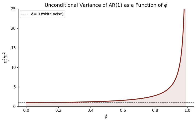
The unconditional variance of an AR(1) is \(\sigma_y^2 = \sigma^2 / (1 - \phi^2)\), which increases sharply as \(\phi \to 1\).

phi_grid = np.linspace(0, 0.99, 200)
variance = 1 / (1 - phi_grid**2)

fig, ax = plt.subplots(figsize=(8, 5))
ax.plot(phi_grid, variance, color=UOE_RED, lw=2.5)
ax.fill_between(phi_grid, variance, alpha=0.1, color=UOE_RED)
ax.set_xlabel('$\\phi$')
ax.set_ylabel('$\\sigma_y^2 / \\sigma^2$')
ax.set_title('Unconditional Variance of AR(1) as a Function of $\\phi$')
ax.set_ylim(0, 25)
ax.axhline(1, ls='--', color=UOE_GREY, lw=1, label='$\\phi = 0$ (white noise)')
ax.legend()
plt.tight_layout()
plt.show()

Exercises

Exercise 1: Simulate an ARMA(2,1) and use ACF/PACF to identify the order.

proc = ArmaProcess(ar=[1, -0.6, -0.2], ma=[1, 0.4])
y = proc.generate_sample(nsample=500)
fig, (ax1, ax2) = plt.subplots(1, 2, figsize=(12, 4))
plot_acf(y, lags=25, ax=ax1)
plot_pacf(y, lags=25, ax=ax2)
plt.show()
# Both ACF and PACF decay → ARMA model