Week 7 — State Space Models & the Kalman Filter

State space models separate the observation equation (what we see) from the state equation (what drives the system). The Kalman filter provides the optimal recursive estimator for the unobserved state.

import matplotlib as mpl
import matplotlib.pyplot as plt
import numpy as np

# Edinburgh palette
UOE_RED   = '#7A2318'
UOE_GOLD  = '#B8860B'
UOE_BLUE  = '#2a78d6'
UOE_GREY  = '#52514e'
COLOURS   = [UOE_RED, UOE_BLUE, UOE_GOLD, '#2ca02c', '#9467bd', '#e377c2']

mpl.rcParams.update({
    'figure.figsize': (10, 5),
    'axes.prop_cycle': mpl.cycler(color=COLOURS),
    'axes.spines.top': False, 'axes.spines.right': False,
    'axes.labelsize': 12, 'axes.titlesize': 14,
    'font.size': 11, 'legend.fontsize': 10,
    'lines.linewidth': 2,
})
print("Plotting style set ✓")

Plotting style set ✓

7.1 The Linear Gaussian State Space Model

State equation: \(\alpha_{t+1} = T \alpha_t + R \eta_t, \quad \eta_t \sim N(0, Q)\)

Observation equation: \(y_t = Z \alpha_t + \varepsilon_t, \quad \varepsilon_t \sim N(0, H)\)

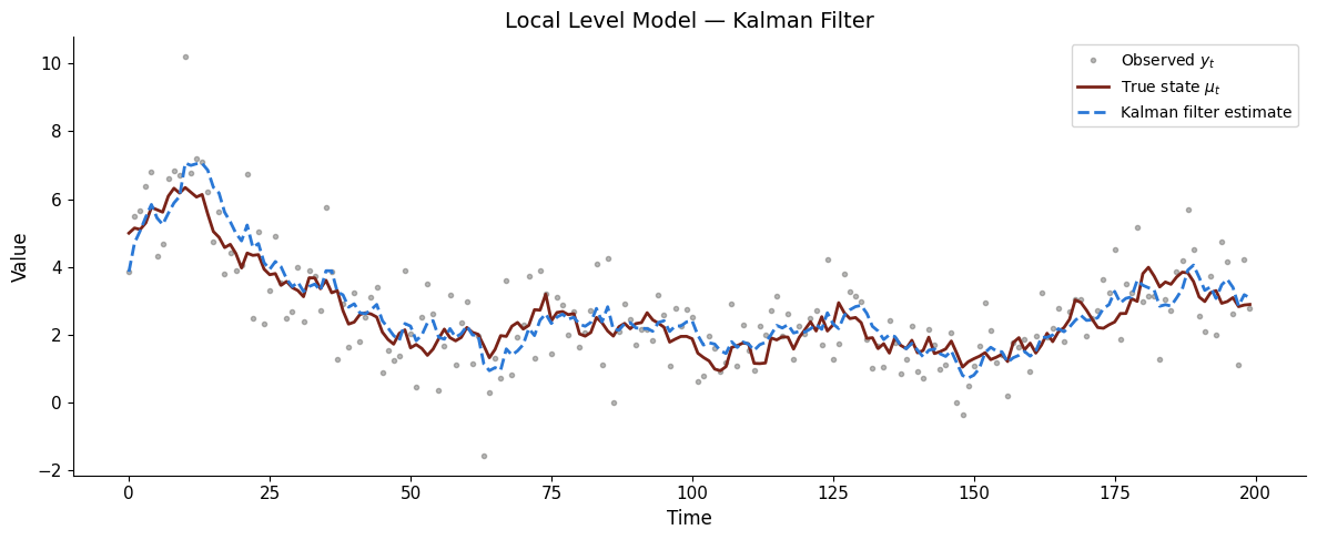
7.2 Local Level Model (Random Walk + Noise)

The simplest state space model: \[y_t = \mu_t + \varepsilon_t, \quad \mu_{t+1} = \mu_t + \eta_t\]

import statsmodels.api as sm

# Simulate local level model
np.random.seed(42)
T = 200
sigma_eta = 0.3  # state noise
sigma_eps = 1.0  # observation noise

mu = np.zeros(T)
y = np.zeros(T)
mu[0] = 5
for t in range(1, T):
    mu[t] = mu[t-1] + np.random.normal(0, sigma_eta)
y = mu + np.random.normal(0, sigma_eps, T)

# Estimate with Kalman filter
mod = sm.tsa.UnobservedComponents(y, level='local level')
res = mod.fit(disp=False)
filtered_state = res.filtered_state[0]

fig, ax = plt.subplots(figsize=(12, 5))
ax.plot(y, 'o', color=UOE_GREY, alpha=0.4, markersize=3, label='Observed $y_t$')
ax.plot(mu, color=UOE_RED, lw=2, label='True state $\\mu_t$')
ax.plot(filtered_state, '--', color=UOE_BLUE, lw=2, label='Kalman filter estimate')
ax.set_xlabel('Time')
ax.set_ylabel('Value')
ax.set_title('Local Level Model — Kalman Filter')
ax.legend()
plt.tight_layout()
plt.show()

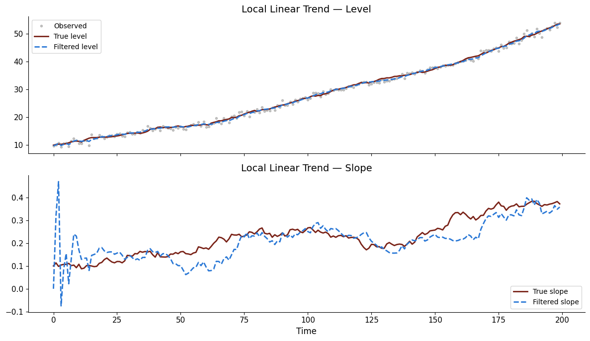
7.3 Local Linear Trend Model

Adds a stochastic slope: \[\mu_{t+1} = \mu_t + \nu_t + \eta_t, \quad \nu_{t+1} = \nu_t + \zeta_t\]

np.random.seed(10)
T = 200
mu2 = np.zeros(T)
nu = np.zeros(T)
mu2[0], nu[0] = 10, 0.1
for t in range(1, T):
    nu[t] = nu[t-1] + np.random.normal(0, 0.01)
    mu2[t] = mu2[t-1] + nu[t-1] + np.random.normal(0, 0.2)
y2 = mu2 + np.random.normal(0, 0.8, T)

mod2 = sm.tsa.UnobservedComponents(y2, level='local linear trend')
res2 = mod2.fit(disp=False)

fig, (ax1, ax2) = plt.subplots(2, 1, figsize=(12, 7), sharex=True)

ax1.plot(y2, 'o', color=UOE_GREY, alpha=0.3, markersize=3, label='Observed')
ax1.plot(mu2, color=UOE_RED, lw=2, label='True level')
ax1.plot(res2.filtered_state[0], '--', color=UOE_BLUE, lw=2, label='Filtered level')
ax1.set_title('Local Linear Trend — Level')
ax1.legend()

ax2.plot(nu, color=UOE_RED, lw=2, label='True slope')
ax2.plot(res2.filtered_state[1], '--', color=UOE_BLUE, lw=2, label='Filtered slope')
ax2.set_title('Local Linear Trend — Slope')
ax2.set_xlabel('Time')
ax2.legend()

plt.tight_layout()
plt.show()

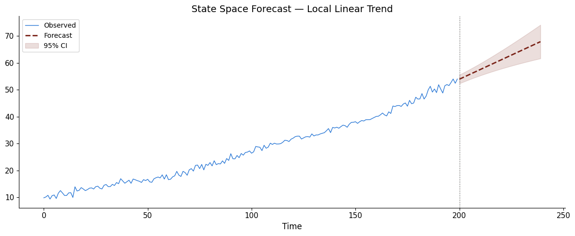
7.4 Forecasting with State Space Models

# Forecast from the local linear trend model
fc2 = res2.get_forecast(steps=40)
ci2 = fc2.conf_int(alpha=0.05)

fig, ax = plt.subplots(figsize=(12, 5))
ax.plot(range(T), y2, color=UOE_BLUE, lw=1, label='Observed')
ax.plot(range(T, T+40), fc2.predicted_mean, '--', color=UOE_RED, lw=2, label='Forecast')
ax.fill_between(range(T, T+40), ci2.values[:, 0] if hasattr(ci2, 'values') else ci2[:, 0], ci2.values[:, 1] if hasattr(ci2, 'values') else ci2[:, 1],
                alpha=0.15, color=UOE_RED, label='95% CI')
ax.axvline(T, ls=':', color=UOE_GREY, lw=1)
ax.set_title('State Space Forecast — Local Linear Trend')
ax.set_xlabel('Time')
ax.legend()
plt.tight_layout()
plt.show()

Exercises

Exercise 1: Add a seasonal component to the state space model.

mod_s = sm.tsa.UnobservedComponents(y_hw, level='local linear trend',
                                     seasonal=12)
res_s = mod_s.fit(disp=False)
res_s.plot_components(figsize=(12, 10))
plt.show()