When we have many time series (GDP, employment, industrial production, …), a small number of common factors may drive them all. Dynamic factor models extract these latent factors.
import matplotlib as mplimport matplotlib.pyplot as pltimport numpy as np# Edinburgh paletteUOE_RED ='#7A2318'UOE_GOLD ='#B8860B'UOE_BLUE ='#2a78d6'UOE_GREY ='#52514e'COLOURS = [UOE_RED, UOE_BLUE, UOE_GOLD, '#2ca02c', '#9467bd', '#e377c2']mpl.rcParams.update({'figure.figsize': (10, 5),'axes.prop_cycle': mpl.cycler(color=COLOURS),'axes.spines.top': False, 'axes.spines.right': False,'axes.labelsize': 12, 'axes.titlesize': 14,'font.size': 11, 'legend.fontsize': 10,'lines.linewidth': 2,})print("Plotting style set ✓")
Plotting style set ✓
8.1 The Idea: Dimension Reduction for Time Series
\[y_{it} = \lambda_i' f_t + e_{it}\]
where \(f_t\) is a \(k\)-dimensional vector of factors and \(\lambda_i\) are loadings.
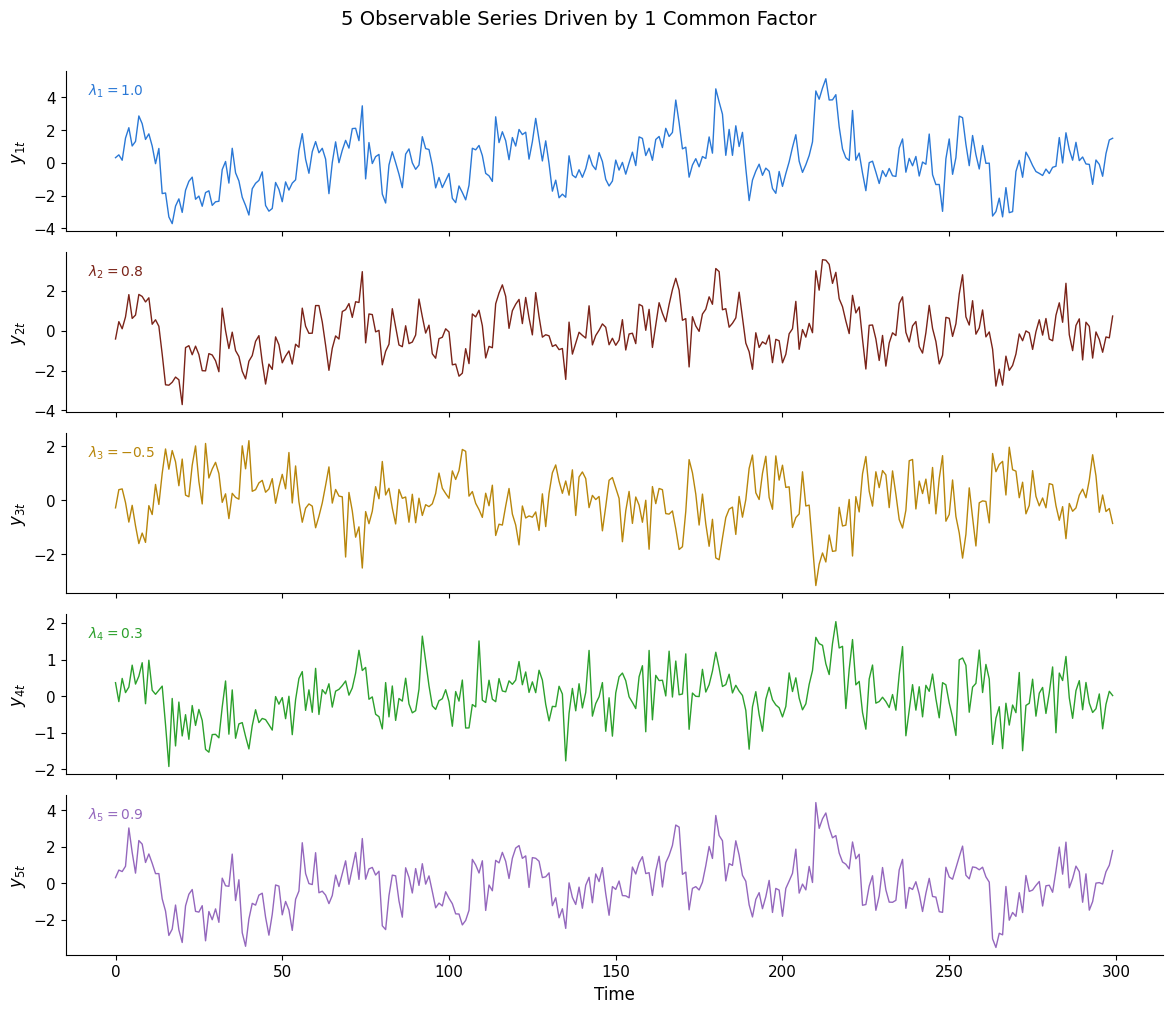
# Simulate a dynamic factor model: 1 factor driving 5 seriesnp.random.seed(42)T =300k =1# number of factors# Factor follows AR(1)factor = np.zeros(T)for t inrange(1, T): factor[t] =0.8* factor[t-1] + np.random.normal(0, 1)# Loadings and idiosyncratic errorsn_series =5loadings = np.array([1.0, 0.8, -0.5, 0.3, 0.9])Y = np.outer(factor, loadings) + np.random.normal(0, 0.5, (T, n_series))fig, axes = plt.subplots(5, 1, figsize=(12, 10), sharex=True)colours = [UOE_BLUE, UOE_RED, UOE_GOLD, '#2ca02c', '#9467bd']for i, (ax, col) inenumerate(zip(axes, colours)): ax.plot(Y[:, i], color=col, lw=1) ax.set_ylabel(f'$y_{{{i+1}t}}$') ax.text(0.02, 0.85, f'$\\lambda_{i+1} = {loadings[i]}$', transform=ax.transAxes, fontsize=10, color=col)axes[-1].set_xlabel('Time')plt.suptitle('5 Observable Series Driven by 1 Common Factor', fontsize=14, y=1.01)plt.tight_layout()plt.show()