Optimisation & Mathematical Methods for Economics The University of Edinburgh · School of Economics
This notebook reviews the core mathematical building blocks you will need throughout the course: sets, functions, vectors, matrices, and key linear algebra concepts. We pair each idea with Python/NumPy code so you can compute and visualise as you learn.
1. Sets and Real Analysis Essentials
A set is a collection of distinct objects. In economics we work mostly with subsets of \(\mathbb{R}^n\).
Key definitions: - Open set: A set \(S\) is open if for every \(x \in S\) there exists \(\varepsilon > 0\) such that \(B(x, \varepsilon) \subset S\). - Closed set: A set is closed if its complement is open, or equivalently if it contains all its limit points. - Bounded set:\(S\) is bounded if there exists \(M > 0\) such that \(\|x\| \leq M\) for all \(x \in S\). - Compact set: A set that is both closed and bounded (in \(\mathbb{R}^n\), by the Heine–Borel theorem).
Why this matters for optimisation: The Extreme Value Theorem guarantees that a continuous function on a compact set attains its maximum and minimum.
For a square matrix \(A\), a scalar \(\lambda\) is an eigenvalue if \(A\mathbf{v} = \lambda \mathbf{v}\) for some non-zero vector \(\mathbf{v}\) (the eigenvector).
A symmetric matrix \(A\) is: - Positive definite if all eigenvalues \(> 0\) (equivalently, \(\mathbf{x}^T A \mathbf{x} > 0\) for all \(\mathbf{x} \neq 0\)) - Positive semi-definite if all eigenvalues \(\geq 0\) - Negative definite if all eigenvalues \(< 0\)
Why this matters: The Hessian matrix being negative definite at a critical point confirms a local maximum.
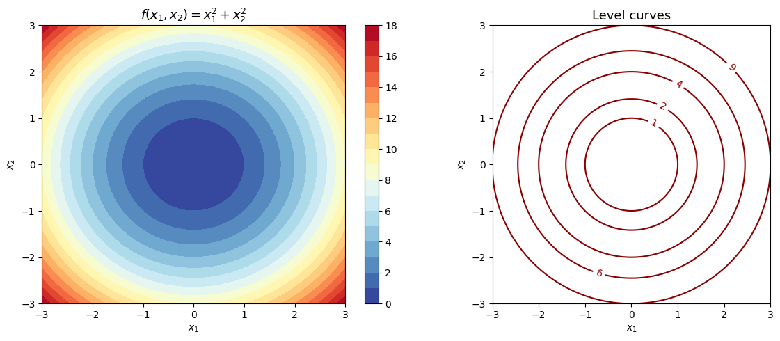
A function \(f: \mathbb{R}^n \to \mathbb{R}\) maps vectors to scalars. In economics, utility functions \(u(x_1, x_2)\) and production functions \(f(K, L)\) are key examples.
Level curves (or indifference curves) are the sets \(\{\mathbf{x} : f(\mathbf{x}) = c\}\) for constant \(c\).