Week 3 — Unconstrained Optimisation II

Gradient Descent & Newton’s Method

Optimisation & Mathematical Methods for Economics The University of Edinburgh · School of Economics

---

This week we move from conditions for optima to algorithms that find them. We implement gradient descent and Newton’s method, compare their convergence, and apply them to economic problems.

1. Gradient Descent

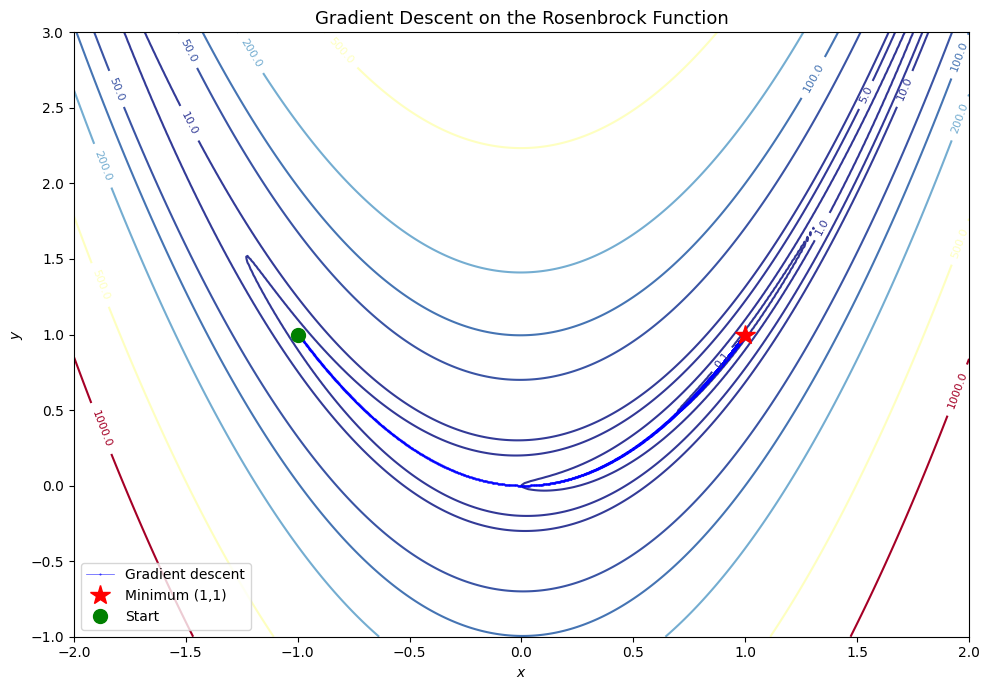
Idea: Start at some \(\mathbf{x}_0\). At each step, move in the direction of steepest descent (negative gradient):

\[\mathbf{x}_{k+1} = \mathbf{x}_k - \alpha \nabla f(\mathbf{x}_k)\]

where \(\alpha > 0\) is the step size (or learning rate).

For minimisation: follow \(-\nabla f\). For maximisation: follow \(+\nabla f\).

import numpy as np
import matplotlib.pyplot as plt

# Minimise the Rosenbrock function: f(x,y) = (1-x)^2 + 100(y-x^2)^2
def rosenbrock(x):
    return (1 - x[0])**2 + 100*(x[1] - x[0]**2)**2

def grad_rosenbrock(x):
    dfdx = -2*(1 - x[0]) + 100*2*(x[1] - x[0]**2)*(-2*x[0])
    dfdy = 100*2*(x[1] - x[0]**2)
    return np.array([dfdx, dfdy])

# Gradient descent
def gradient_descent(grad_f, x0, alpha=0.001, tol=1e-6, max_iter=10000):
    x = x0.copy()
    path = [x.copy()]
    for i in range(max_iter):
        g = grad_f(x)
        if np.linalg.norm(g) < tol:
            break
        x = x - alpha * g
        path.append(x.copy())
    return np.array(path)

x0 = np.array([-1.0, 1.0])
path_gd = gradient_descent(grad_rosenbrock, x0, alpha=0.001, max_iter=20000)

print(f"Gradient descent: {len(path_gd)} iterations")
print(f"Final point: ({path_gd[-1][0]:.4f}, {path_gd[-1][1]:.4f})")
print(f"Final f value: {rosenbrock(path_gd[-1]):.6f}")

Gradient descent: 20001 iterations
Final point: (0.9999, 0.9997)
Final f value: 0.000000

# Visualise the path
x1 = np.linspace(-2, 2, 300)
x2 = np.linspace(-1, 3, 300)
X1, X2 = np.meshgrid(x1, x2)
Z = (1 - X1)**2 + 100*(X2 - X1**2)**2

fig, ax = plt.subplots(figsize=(10, 7))
levels = [0.1, 1, 5, 10, 50, 100, 200, 500, 1000]
cs = ax.contour(X1, X2, Z, levels=levels, cmap='RdYlBu_r')
ax.clabel(cs, inline=True, fontsize=8)
ax.plot(path_gd[:, 0], path_gd[:, 1], 'b.-', markersize=1, linewidth=0.5,
        alpha=0.7, label='Gradient descent')
ax.plot(1, 1, 'r*', markersize=15, label='Minimum (1,1)')
ax.plot(x0[0], x0[1], 'go', markersize=10, label='Start')
ax.set_xlabel('$x$'); ax.set_ylabel('$y$')
ax.set_title("Gradient Descent on the Rosenbrock Function", fontsize=13)
ax.legend()
plt.tight_layout()
plt.show()

2. Newton’s Method

Newton’s method uses second-order information (the Hessian) for faster convergence:

\[\mathbf{x}_{k+1} = \mathbf{x}_k - [H_f(\mathbf{x}_k)]^{-1} \nabla f(\mathbf{x}_k)\]

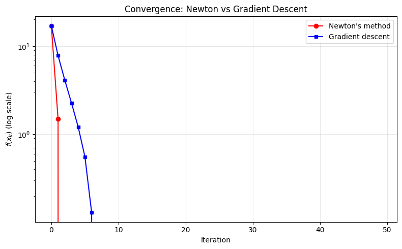
Convergence: Newton’s method has quadratic convergence near the optimum (vs. linear for gradient descent), but each step is more expensive and requires computing/inverting the Hessian.

# Newton's method for a simpler example: f(x,y) = x^4 + y^4 - 4xy + 1
def f_simple(x):
    return x[0]**4 + x[1]**4 - 4*x[0]*x[1] + 1

def grad_simple(x):
    return np.array([4*x[0]**3 - 4*x[1], 4*x[1]**3 - 4*x[0]])

def hess_simple(x):
    return np.array([[12*x[0]**2, -4],
                     [-4, 12*x[1]**2]])

def newtons_method(grad_f, hess_f, x0, tol=1e-8, max_iter=100):
    x = x0.copy()
    path = [x.copy()]
    for i in range(max_iter):
        g = grad_f(x)
        if np.linalg.norm(g) < tol:
            break
        H = hess_f(x)
        direction = np.linalg.solve(H, -g)
        x = x + direction
        path.append(x.copy())
    return np.array(path)

x0 = np.array([2.0, 2.0])

# Compare
path_newton = newtons_method(grad_simple, hess_simple, x0)
path_gd2 = gradient_descent(grad_simple, x0, alpha=0.01, max_iter=500)

print(f"Newton: {len(path_newton)} iterations -> ({path_newton[-1][0]:.6f}, {path_newton[-1][1]:.6f})")
print(f"GD:     {len(path_gd2)} iterations -> ({path_gd2[-1][0]:.6f}, {path_gd2[-1][1]:.6f})")

Newton: 7 iterations -> (1.000000, 1.000000)
GD:     183 iterations -> (1.000000, 1.000000)

# Convergence comparison
fig, ax = plt.subplots(figsize=(8, 5))
fvals_newton = [f_simple(p) for p in path_newton]
fvals_gd = [f_simple(p) for p in path_gd2]
ax.semilogy(range(len(fvals_newton)), fvals_newton, 'r-o', label="Newton's method", markersize=6)
ax.semilogy(range(min(50, len(fvals_gd))), fvals_gd[:50], 'b-s', label='Gradient descent', markersize=4)
ax.set_xlabel('Iteration'); ax.set_ylabel('$f(x_k)$ (log scale)')
ax.set_title('Convergence: Newton vs Gradient Descent')
ax.legend(); ax.grid(True, alpha=0.3)
plt.tight_layout()
plt.show()

3. Quasi-Newton Methods: BFGS

Computing the full Hessian is expensive. BFGS (Broyden–Fletcher–Goldfarb–Shanno) approximates the inverse Hessian using gradient information only, achieving superlinear convergence without second derivatives.

In practice, BFGS (and its limited-memory variant L-BFGS) is the workhorse of smooth optimisation.

from scipy.optimize import minimize

# Using scipy's BFGS
x0 = np.array([2.0, 2.0])
result = minimize(f_simple, x0, method='BFGS', jac=grad_simple)
print("BFGS result:")
print(f"  x* = ({result.x[0]:.6f}, {result.x[1]:.6f})")
print(f"  f* = {result.fun:.6f}")
print(f"  Iterations: {result.nit}")
print(f"  Gradient evaluations: {result.njev}")

BFGS result:
  x* = (1.000000, 1.000000)
  f* = -1.000000
  Iterations: 7
  Gradient evaluations: 8

Exercises

Exercise 1: Implement gradient descent for \(f(x,y) = (x-3)^2 + 2(y+1)^2\). Try different step sizes \(\alpha \in \{0.01, 0.1, 0.5, 1.0\}\) and plot the convergence.

def f_quad(x): return (x[0]-3)**2 + 2*(x[1]+1)**2
def grad_quad(x): return np.array([2*(x[0]-3), 4*(x[1]+1)])

for alpha in [0.01, 0.1, 0.5, 1.0]:
    path = gradient_descent(grad_quad, np.array([0.0, 0.0]), alpha=alpha, max_iter=200)
    fvals = [f_quad(p) for p in path]
    plt.semilogy(fvals, label=f'alpha={alpha}')
plt.legend(); plt.xlabel('Iteration'); plt.ylabel('f(x)')
plt.title('Effect of step size'); plt.show()
# alpha=0.5 converges fastest; alpha=1.0 diverges (too large)

Exercise 2: Use scipy.optimize.minimize with method=‘Nelder-Mead’ (derivative-free) and compare with BFGS. When might a derivative-free method be useful?

Derivative-free methods are useful when the objective is noisy, non-differentiable, or the gradient is very expensive to compute (e.g., simulation-based models in macroeconomics).