Week 7 — Linear Programming

The Simplex Method & Economic Models

Optimisation & Mathematical Methods for Economics The University of Edinburgh · School of Economics

---

Linear programming (LP) is the workhorse of operations research and has deep connections to economics through duality, shadow prices, and input–output models.

1. Standard Form and Geometry

A linear program in standard form:

\[\min \mathbf{c}^T \mathbf{x} \quad \text{s.t.} \quad A\mathbf{x} \leq \mathbf{b}, \quad \mathbf{x} \geq \mathbf{0}\]

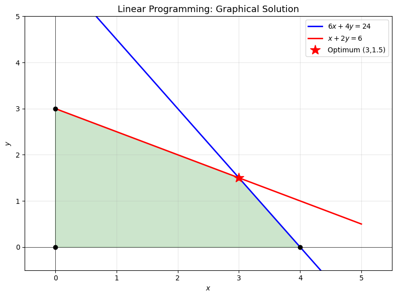
Fundamental theorem of LP: If an LP has an optimal solution, there is one at a vertex (extreme point) of the feasible polyhedron.

import numpy as np
import matplotlib.pyplot as plt
from scipy.optimize import linprog

# LP: Maximise 5x + 4y subject to:
# 6x + 4y <= 24, x + 2y <= 6, x,y >= 0
# (linprog minimises, so we negate the objective)

c = [-5, -4]
A_ub = [[6, 4], [1, 2]]
b_ub = [24, 6]

result = linprog(c, A_ub=A_ub, b_ub=b_ub, bounds=[(0,None),(0,None)])
print(f"Optimal x = {result.x[0]:.2f}, y = {result.x[1]:.2f}")
print(f"Maximum value = {-result.fun:.2f}")

# Visualise
fig, ax = plt.subplots(figsize=(8, 6))
x = np.linspace(0, 5, 200)

# Constraints
ax.plot(x, (24-6*x)/4, 'b-', label='$6x+4y=24$', linewidth=2)
ax.plot(x, (6-x)/2, 'r-', label='$x+2y=6$', linewidth=2)
ax.axhline(0, color='k', linewidth=0.5)
ax.axvline(0, color='k', linewidth=0.5)

# Feasible region
from matplotlib.patches import Polygon
vertices = np.array([[0,0],[4,0],[3,1.5],[0,3]])
poly = Polygon(vertices, alpha=0.2, color='green')
ax.add_patch(poly)

# Vertices and optimum
for v in vertices:
    ax.plot(v[0], v[1], 'ko', markersize=6)
ax.plot(result.x[0], result.x[1], 'r*', markersize=15, label=f'Optimum ({result.x[0]:.0f},{result.x[1]:.1f})')

ax.set_xlim(-0.5, 5.5); ax.set_ylim(-0.5, 5)
ax.set_xlabel('$x$'); ax.set_ylabel('$y$')
ax.set_title('Linear Programming: Graphical Solution', fontsize=13)
ax.legend(); ax.grid(True, alpha=0.3)
plt.tight_layout()
plt.show()

Optimal x = 3.00, y = 1.50
Maximum value = 21.00

2. LP Duality and Shadow Prices

Every LP has a dual problem. If the primal is \(\min \mathbf{c}^T\mathbf{x}\) s.t. \(A\mathbf{x} \geq \mathbf{b}\), \(\mathbf{x} \geq 0\), the dual is \(\max \mathbf{b}^T\mathbf{y}\) s.t. \(A^T\mathbf{y} \leq \mathbf{c}\), \(\mathbf{y} \geq 0\).

Strong duality: optimal primal value = optimal dual value.

The dual variables are shadow prices — the rate of change of the optimal value with respect to the constraint bounds.

# LP with PuLP — the diet problem
try:
    from pulp import *
except ImportError:
    import subprocess
    subprocess.check_call(['pip', 'install', 'pulp', '-q', '--break-system-packages'])
    from pulp import *

# Minimise cost of a diet meeting nutritional requirements
# Foods: bread, milk, cheese
prob = LpProblem("Diet", LpMinimize)

bread = LpVariable("bread", 0)   # servings
milk = LpVariable("milk", 0)
cheese = LpVariable("cheese", 0)

# Costs per serving
prob += 2*bread + 3.5*milk + 5*cheese, "Total cost"

# Nutritional constraints (minimum daily requirements)
prob += 3*bread + 8*milk + 6*cheese >= 50, "Protein"     # grams
prob += 250*bread + 300*milk + 100*cheese >= 2000, "Calories"
prob += 2*bread + 10*milk + 8*cheese >= 30, "Calcium"     # mg

prob.solve(PULP_CBC_CMD(msg=0))

print(f"Status: {LpStatus[prob.status]}")
print(f"Optimal diet:")
for v in prob.variables():
    print(f"  {v.name}: {v.varValue:.2f} servings")
print(f"Minimum daily cost: ${value(prob.objective):.2f}")

Status: Optimal
Optimal diet:
  bread: 0.91 servings
  cheese: 0.00 servings
  milk: 5.91 servings
Minimum daily cost: $22.50

Exercises

Exercise 1: A firm can produce 2 goods. Good 1 uses 2 hours of labour and 1 unit of capital; Good 2 uses 1 hour of labour and 3 units of capital. Available: 100 hours of labour, 90 units of capital. Profits: $30 per unit of Good 1, $50 per unit of Good 2. Formulate and solve as an LP. What are the shadow prices?

from scipy.optimize import linprog
c = [-30, -50]  # negate for minimisation
A = [[2, 1], [1, 3]]
b = [100, 90]
res = linprog(c, A_ub=A, b_ub=b, bounds=[(0,None),(0,None)])
print(f"x1={res.x[0]:.1f}, x2={res.x[1]:.1f}, profit=${-res.fun:.0f}")