Week 9 — Dynamic Optimisation II

Dynamic Programming & the Bellman Equation

Optimisation & Mathematical Methods for Economics The University of Edinburgh · School of Economics

Dynamic programming (Bellman, 1957) transforms an infinite-horizon sequential decision problem into a functional equation. This connects directly to the value function iteration you study in Programming & Numerical Methods.

1. The Bellman Equation

The agent solves: \(V(k) = \max_c \{ u(c) + \beta V(k') \}\) subject to \(k' = f(k) - c\).

Principle of optimality: An optimal policy has the property that regardless of the initial state and initial decision, the remaining decisions must constitute an optimal policy.

Contraction mapping theorem: Under standard assumptions, the Bellman operator \(T\) is a contraction. Iterating \(V_{n+1} = TV_n\) from any initial guess converges to the unique fixed point \(V^*\).

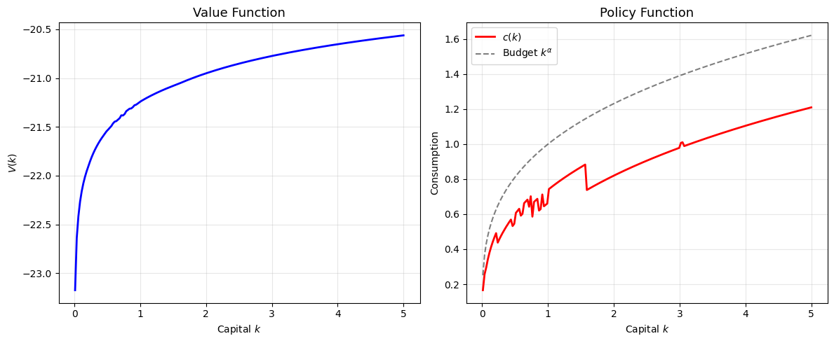
import numpy as np
import matplotlib.pyplot as plt

# Value function iteration for a consumption-savings problem
# V(k) = max_c { u(c) + beta * V(k') }
# k' = k^alpha - c (no depreciation for simplicity)

alpha = 0.3
beta = 0.96
n_k = 200
k_grid = np.linspace(0.01, 5, n_k)
V = np.zeros(n_k)  # initial guess

tol = 1e-6
max_iter = 500

for iteration in range(max_iter):
    V_new = np.zeros(n_k)
    policy = np.zeros(n_k, dtype=int)

    for i, k in enumerate(k_grid):
        budget = k**alpha
        # All feasible consumption levels
        c_candidates = budget - k_grid[k_grid <= budget * 0.999]
        if len(c_candidates) == 0:
            continue
        # Find the k' index for each c
        kp_indices = np.searchsorted(k_grid, budget - c_candidates) - 1
        kp_indices = np.clip(kp_indices, 0, n_k-1)
        # Bellman
        values = np.log(np.maximum(c_candidates, 1e-10)) + beta * V[kp_indices]
        best = np.argmax(values)
        V_new[i] = values[best]
        policy[i] = kp_indices[best]

    if np.max(np.abs(V_new - V)) < tol:
        print(f"Converged in {iteration+1} iterations")
        break
    V = V_new.copy()

# Plot value function and policy function
fig, axes = plt.subplots(1, 2, figsize=(12, 5))

axes[0].plot(k_grid, V, 'b-', linewidth=2)
axes[0].set_xlabel('Capital $k$'); axes[0].set_ylabel('$V(k)$')
axes[0].set_title('Value Function', fontsize=13)
axes[0].grid(True, alpha=0.3)

c_policy = k_grid**alpha - k_grid[policy]
axes[1].plot(k_grid, c_policy, 'r-', linewidth=2, label='$c(k)$')
axes[1].plot(k_grid, k_grid**alpha, 'k--', alpha=0.5, label='Budget $k^\\alpha$')
axes[1].set_xlabel('Capital $k$'); axes[1].set_ylabel('Consumption')
axes[1].set_title('Policy Function', fontsize=13)
axes[1].legend(); axes[1].grid(True, alpha=0.3)

plt.tight_layout()
plt.show()

Converged in 337 iterations

2. Analytical Solution: Log Utility + Cobb-Douglas

With \(u(c)=\ln c\) and \(f(k)=k^\alpha\), the value function has the closed form:

\[V(k) = \frac{\alpha \beta}{(1-\alpha\beta)} \ln k + \text{const}\]

and the optimal savings rate is \(s = \alpha \beta\), giving \(c^* = (1-\alpha\beta)k^\alpha\).

# Compare numerical solution to analytical
s_analytical = alpha * beta
c_analytical = (1 - alpha*beta) * k_grid**alpha

fig, ax = plt.subplots(figsize=(8, 5))
ax.plot(k_grid, c_policy, 'r-', linewidth=2, label='Numerical VFI')
ax.plot(k_grid, c_analytical, 'b--', linewidth=2, label='Analytical')
ax.set_xlabel('Capital $k$'); ax.set_ylabel('Consumption $c(k)$')
ax.set_title('Policy Function: Numerical vs Analytical', fontsize=13)
ax.legend(); ax.grid(True, alpha=0.3)
plt.tight_layout()
plt.show()

max_err = np.max(np.abs(c_policy - c_analytical))
print(f"Maximum error: {max_err:.6f}")
print(f"Analytical savings rate: {s_analytical:.4f}")

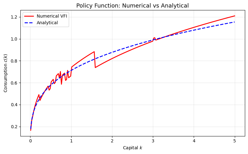
Maximum error: 0.080234
Analytical savings rate: 0.2880

Exercises

Exercise 1: Modify the VFI code to add a borrowing constraint \(k' \geq \underline{k}\). How does the policy function change?

Add k_min = 0.5 and change the feasible set to k_grid[(k_grid >= k_min) & (k_grid <= budget)]. The policy function will be flatter near the constraint — consumption drops because the agent cannot borrow.