Week 10 — Frontiers

Stochastic Optimisation, Machine Learning & Beyond

Optimisation & Mathematical Methods for Economics The University of Edinburgh · School of Economics

---

This final week surveys three frontiers where optimisation meets modern economics and data science: stochastic dynamic programming, stochastic gradient descent for machine learning, and Bayesian optimisation for simulation-based models.

1. Stochastic Dynamic Programming

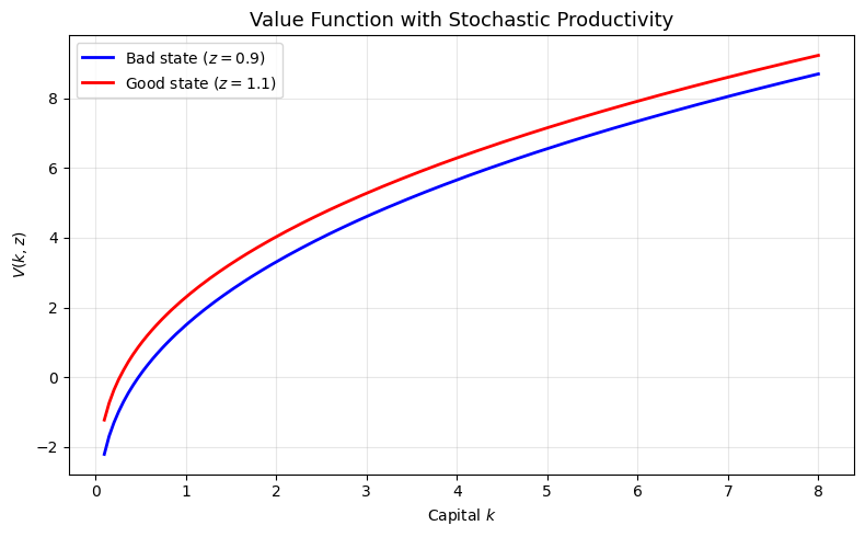
Real economies face uncertainty. The Bellman equation becomes:

\[V(k, z) = \max_c \{ u(c) + \beta \, \mathbb{E}[V(k', z') \mid z] \}\]

where \(z\) is a stochastic productivity shock following a Markov process.

import numpy as np
import matplotlib.pyplot as plt

# Stochastic growth model with 2-state Markov productivity
alpha, beta, delta = 0.3, 0.96, 0.05
z_vals = np.array([0.9, 1.1])   # bad / good state
P = np.array([[0.8, 0.2],       # transition matrix
              [0.2, 0.8]])

n_k, n_z = 150, 2
k_grid = np.linspace(0.1, 8, n_k)
V = np.zeros((n_k, n_z))

for iteration in range(500):
    V_new = np.zeros_like(V)
    for iz, z in enumerate(z_vals):
        for ik, k in enumerate(k_grid):
            budget = z * k**alpha + (1-delta)*k
            c_vals = budget - k_grid[k_grid < budget*0.99]
            if len(c_vals) == 0:
                continue
            kp_idx = np.searchsorted(k_grid, budget - c_vals) - 1
            kp_idx = np.clip(kp_idx, 0, n_k-1)
            EV = P[iz] @ V[kp_idx].T
            vals = np.log(np.maximum(c_vals, 1e-10)) + beta * EV
            V_new[ik, iz] = np.max(vals)
    if np.max(np.abs(V_new - V)) < 1e-6:
        print(f"Converged in {iteration+1} iterations")
        break
    V = V_new.copy()

fig, ax = plt.subplots(figsize=(8, 5))
ax.plot(k_grid, V[:, 0], 'b-', linewidth=2, label='Bad state ($z=0.9$)')
ax.plot(k_grid, V[:, 1], 'r-', linewidth=2, label='Good state ($z=1.1$)')
ax.set_xlabel('Capital $k$'); ax.set_ylabel('$V(k,z)$')
ax.set_title('Value Function with Stochastic Productivity', fontsize=13)
ax.legend(); ax.grid(True, alpha=0.3)
plt.tight_layout()
plt.show()

Converged in 294 iterations

2. Stochastic Gradient Descent (SGD)

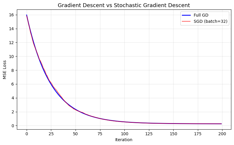
In machine learning, the objective is an expectation over data:

\[\min_\theta \frac{1}{N} \sum_{i=1}^N \ell(\theta; x_i, y_i)\]

SGD approximates the gradient using a random mini-batch rather than all \(N\) samples:

\[\theta_{t+1} = \theta_t - \alpha_t \nabla \ell(\theta_t; x_i, y_i)\]

Variants: momentum, Adam, RMSProp — all trade off noise reduction against convergence speed.

# SGD for linear regression
np.random.seed(42)
n, d = 1000, 5
X = np.random.randn(n, d)
true_theta = np.array([1, -2, 0.5, 3, -1.5])
y = X @ true_theta + 0.5*np.random.randn(n)

# Full gradient descent vs SGD
theta_gd = np.zeros(d)
theta_sgd = np.zeros(d)
lr = 0.01
batch_size = 32

losses_gd, losses_sgd = [], []

for t in range(200):
    # Full GD
    grad_full = (2/n) * X.T @ (X @ theta_gd - y)
    theta_gd -= lr * grad_full
    losses_gd.append(np.mean((X @ theta_gd - y)**2))

    # SGD
    idx = np.random.choice(n, batch_size, replace=False)
    grad_batch = (2/batch_size) * X[idx].T @ (X[idx] @ theta_sgd - y[idx])
    theta_sgd -= lr * grad_batch
    losses_sgd.append(np.mean((X @ theta_sgd - y)**2))

fig, ax = plt.subplots(figsize=(8, 5))
ax.plot(losses_gd, 'b-', linewidth=2, label='Full GD')
ax.plot(losses_sgd, 'r-', alpha=0.7, label=f'SGD (batch={batch_size})')
ax.set_xlabel('Iteration'); ax.set_ylabel('MSE Loss')
ax.set_title('Gradient Descent vs Stochastic Gradient Descent', fontsize=13)
ax.legend(); ax.grid(True, alpha=0.3)
plt.tight_layout()
plt.show()

3. Course Summary

Over 10 weeks we have built a complete optimisation toolkit:

Weeks	Topic	Key result
1	Foundations	Eigenvalues, positive definiteness
2–3	Unconstrained	FOC/SOC, gradient descent, Newton
4–5	Constrained	Lagrange, KKT, complementary slackness
6	Convex	Global optimality, duality, CVXPY
7	Linear programming	Simplex, shadow prices, LP duality
8–9	Dynamic	Euler equation, Bellman, VFI
10	Frontiers	Stochastic DP, SGD, modern methods

These tools underpin virtually every model in modern economics — from consumer choice to DSGE models to machine learning.

Exercises

Exercise 1: Implement SGD with momentum: \(v_{t+1} = \gamma v_t + \alpha \nabla \ell\) and \(\theta_{t+1} = \theta_t - v_{t+1}\). Does it converge faster than vanilla SGD?

theta_mom = np.zeros(d)
v = np.zeros(d)
gamma = 0.9
for t in range(200):
    idx = np.random.choice(n, batch_size)
    grad = (2/batch_size) * X[idx].T @ (X[idx] @ theta_mom - y[idx])
    v = gamma * v + lr * grad
    theta_mom -= v
# Yes, momentum smooths the updates and typically converges faster.